In a previous tutorial blog post, I summarized the bootstrapping routine developed by Sacha Epskamp and me that we recommend for testing the stability / accuracy / precision of estimated network models and parameters1. This matters a great deal and should be considered a standard step in every empirical network paper: Without knowing the uncertainty surrounding statistical parameters such as edge weights or centrality indices, any inference you draw from your estimated networks stands on very shaky ground. The previous blog post was a summary of our tutorial paper on the topic of stability. For an R-tutorial on stability which you can run step by step on your own computer (including data), see for instance here (slides from a workshop I gave in Madrid 2017) or here (Amsterdam Network Analysis summer school; see day 3, lecture “MRF2”). Finally, for an accessible explanation of how to properly interpret bootstrapped regularized coefficients, see here.
Common reasons for stability issues
This blog post is the second part of the series, and highlights issues related to stability or accuracy of network models. It’s largely based on our Tutorial on Regularized Partial Correlation Networks forthcoming in Psychological Methods, and on a recent discussion on Facebook. Many of the points below were raised by Payton Jones, Denny Borsboom, and Sacha Epskamp, so all credit to them. This is just an accessible summary.
As described in the Facebook discussion, there are some reasons for stability problems.
Power
As you know by now, model stability is correlated to power, and power comes from 1) more participants and 2) fewer nodes in the network (because this means you have less parameters to estimate)2. If you have a highly unstable model, with parameters that are all over the place, the reason is probably the same as for factor models, regressions, and t-tests: Too few participants for the parameters you estimate.
Outliers
Outliers can lead to problems, especially in small samples. Remember that the bootstrapping routines we use in the R-package bootnet to look at the stability of your network model resample your data. If parameters differ a lot depending on whether the few people with severe outliers are included in the sample or not, then you might end up with imprecise results3.
Regularization
Network models as currently implemented often use regularization to err on the side of sparsity: This puts edge coefficients exactly to zero. Think about this as some sort of threshold that edges must reach. If they don’t, they are put to zero4. If you have many edges that are just barely above this threshold, and you use bootstrapping routines, it’s likely that each time you estimate your network based on bootstrapped data, different weak edges survive regularization, which will lead to an unstable network.
Related, regularization assumes that your true network is sparse. If this is not the case — i.e. if your true network is dense — and especially in cases when edge weights are similar to each other, this can result in estimation and stability issues.
Centrality
Imagine the results of boostrapping show that your centrality coefficients are estimated unreliably, or, put differently, that each time you take a subsample of your sample, the order of centrality estimates comes out differently. Usually, this implies a problem, and there are many reasons this could come from. The first reason we usually think of is that there is a clear order of centrality in the true model (node A -> node B -> node C -> node D), where A is the most central node, and D the least central node. But there is a second reason that I want to highlight here: imagine you have a strongly connected true network where all 4 nodes are roughly equally central, so A = B = C = D. What happens if you bootstrap this? With every bootstrapping, sampling variability would lead to different centrality orders, and the results would appear highly unstable. When it truth, this instability merely reflects sampling error. Not knowing the true model, there is no way for us to find out, but it seems important to add that information here.
Closeness centrality
Closeness in a network becomes 0 if a network has at least one node that is unconnected to the rest. Imagine you have a very weakly connected network: It is possible that in half of the bootstrapped networks, one node is unconnected. Since we look at the similarity of centrality across bootstraps in bootnet, this would result in a very low stability coefficient. Similarly, since we drop cases in the bootstrapping routines (to determine if the same centrality order emerges when subsetting the data), this can lead to unconnected nodes, which dramatically reduces closeness stability.
Betweenness centrality
Betweenness centrality may be unstable if there are (a) multiple plausible shortest paths connecting for instance two communities X and Y, and if (b) these multiple shortest paths are roughly equally strong.
Here is an example for the situation (codes and full output available here) that Sacha just put together for this blog post; the codes also nicely functions as a tutorial on how to set up your own brief simulation study, using the netSimulator() function we described in our recent tutorial paper on network power estimation.
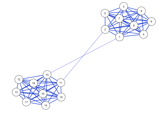
First we create a network structure that has 2 bridges, and simulate a dataset with n=5000. This should give us ample power for stable estimation.

As expected, network estimation looks highly stable; the correlation of the estimated network with the true network is high, and sensitivity and specificity are good (run the codes yourself to see the corresponding plots). The correlation stability for strength centrality is 0.44, meaning you can drop 44% of your dataset and still retain a correlation of about 0.7 between the order of strength centrality in your subsampled data/network and the order of strength centrality in your full data/network.
For Betweenness, however, the centrality stability coefficient is 0. Why? Every time you bootstrap and estimate a network structure, one of the two edges connecting the two communities is likely going to be a tiny bit larger than the other, meaning it has very high betweenness centrality (the node of the other edge get a very small betweenness centrality). This varies across bootstraps, leading to highly unstable betweenness results.
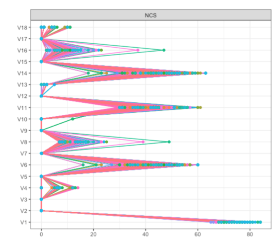
We stumbled across this when analyzing a dataset of about 8000 participants; results are described in detail here (pp. 5 and 6). To investigate this further, we dropped 5% of the sample 1000 times in this dataset, and plotted Betweenness for all items:

As you can see, items V6, V8, V11 and V14 (which were the 4 items forming the two bridges across communities) showed pronounced Betweenness, leading to a centrality correlation coefficient of 0.
Marginal crosstables & skip imputation
When you estimate the correlations of your items as input for the Gaussian Graphical Model5 via polychoric correlations, this can lead to problems in case you have (a) a small dataset and (b) very skewed items / infrequent categories. This leads to zeroes in the marginal crosstables, resulting in unstable results. For instance, here we show bootstrap results of highly unstable edges even though N is high (if you cannot access the paper due to the paywall, see here). Even if this problem does not exist in your raw data, keep in mind that it might be introduced once you start bootstrapping the data, because, as Sacha wrote:
Bootstrapping will reduce entropy, as the collection of all unique outcomes in your bootstrapped dataset is by definition equal or smaller than the collection of all unique outcomes in your raw dataset.
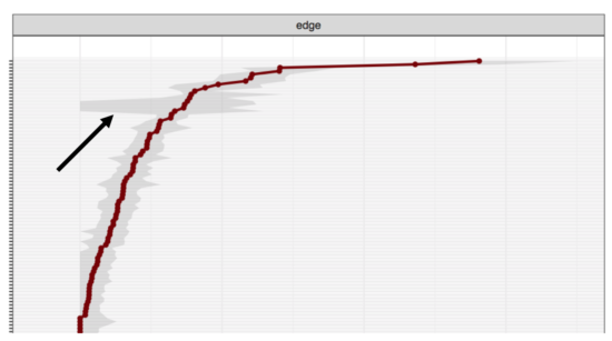
This is related to skip questions. Especially in large epidemiology datasets, it is quite common to skip certain symptoms dependent on others. For instance, if a person does not meet at least one of the two core symptoms for Major Depression, the other 7 secondary symptoms are usually not queried. These missing values are commonly replaced by zeros (zero-imputation), which can lead to considerable problems described in more detail here. These problems are also visible in stability analysis. When we bootstrapped a very large dataset (that we expected to be very stable), we found that the core items that determine skip very extremely unstable (the grey areas in the plot below indicate the 95% CI of the edge weight parameter estimates; x-axis is parameter strength, y-axis the node in question).

Network structure
As Denny Borsboom stated:
The most important dark horse is network structure. Some network structures are very hard to estimate even with massive datasets and others work very well at small sample sizes. E.g. Isingfit has trouble recovering scale free networks even at very high sample sizes, see https://www.nature.com/articles/srep05918.
A scale-free network is a specific type of network structure where the degree distribution follows a power law. The paper reference above shows that IsingFit, the R package developed to estimate Ising Models in psychological data, performs very well if data come from random or small world networks, but does not perform well when data where generated from scale-free networks:
The above pattern of results, involving adequate network recovery with high specificity and moderately high sensitivity, is representative for almost all simulated conditions. The only exception to this rule results when the largest random and scale-free networks (100 nodes) are coupled with the highest level of connectivity. In these cases, the estimated coefficients show poor correlations with the coefficients of the generating networks, even for conditions involving 2000 observations […].
Conclusion
Without stability analysis, inference cannot follow, which is why we previously suggested to adding stability as a third step to the network psychometrics routine: Network estimation, network inference, network stability. But as pointed out in the recent Winter School here in Amsterdam, it makes more sense to change around the order to network estimation, network stability, network inference, for obvious reasons.
There is another benefit to stability analysis: You might not notice that there were problems in the network estimation itself, such as zeroes in the marginal cross-tables, but these often come to light in the stability analysis. As such, you can use the bootnet routines as a way to identify potential issues in your data as well.
- This pertains to between-subjects, psychological network models in cross-sectional data.
- And 3) signal in the data
- This is not a call for removing outliers.
- Not exactly correct, see our tutorial paper for a more accurate description.
- Or a factor model, for that matter … all problems that stem from correlations are equally detrimental to factor models, of course.

Pingback: Looking back at 2018 - Eiko Fried
Pingback: Summary of my academic 2018 - Eiko Fried
Pingback: Tutorial: how to review psychopathology network papers | Psych Networks