In two previous blog posts, we identified a fundamental challenge to community detection in psychometric network analysis: Commonly used algorithms assign each node to one particular community. One of these blog posts was an R tutorial I wrote, the other a guest blog by Tessa Blanken and Marie Deserno on a new method to identify communities.
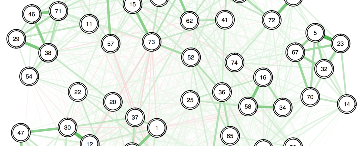
What is the problem? Let’s look at this empirical network of 20 PTSD symptoms:
While the walktrap algorithm—a commonly used method that I described previously—detects 3 communities, we can see that node D2 in the bottom sort of belongs to several communities: while it is assigned to the large red community, it also has a strong connection to D4, which in turn connects to D3. So arguably, D2 is, at least to some degree, also part of that other community.
Many of you will know by now that network models are equivalent to latent variable models under a set of conditions. If you generate data under a 1-factor model, you will find a fully connected network with one giant community. And if you simulate data from a network model that has 3 strong communities that are unconnected, a 3-factor model will describe the data very well. Denny Borsboom has described this from a more theoretical perspective in this guest blog, and Joost Kruis described his statistical paper on the topic in this guest blog.
The advantage of factor models is that they can deal with cross-loadings, i.e. when an item loads on 2 or more factors1:
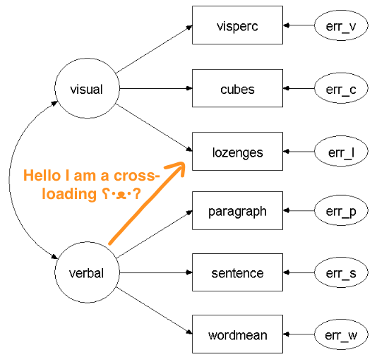
Current community detection methods that do not allow such “cross-loadings” are therefore akin to simple structure in confirmatory factor models where an item can only load on one factor (i.e. belong to one community). And if there is any agreement among psychometricians, then that simple structure is rarely found in psychological data.
Clique Percolation
Enter clique percolation, a well-established method e.g. described in chapter 9 of the free network science book by Barabasi2. Usually, the program cfinder is used for that, which was also used in the network psychometrics paper by Tessa and Marie. Clique percolation allows to identify nodes that belong to multiple communities.
A few days ago, Jens Lange published the R package CliquePercolation on CRAN, and finally we can use clique percolation in R! Jens provided a beautiful and detailed explanation of the package’s functionalities, and I will use some of his code and explanations here in this short tutorial, and apply it to an open clinical dataset.
Clique percolation tutorial
So let’s use empirical data and see how the method performs. Code and data for this tutorial are available here. We use a dataset of 221 military veterans for whom we have 20 PTSD symptoms based on the DSM-5; our empirical paper on this dataset is available here where you can also find more information on the sample composition, measurement of symptoms, etc.
1. PTSD network based on the DSM-5
In a first step, we simply estimate the network structure, using a regularized gaussian graphical model, and use 4 communities based on theory: the 4 communities of symptoms described in the DSM-5.
This can be easily done in R:
load('data.Rdata')

### estimate network
n1 <- estimateNetwork(data, default="EBICglasso")

### plot network
names<-c('B1','B2', 'B3', 'B4', 'B5', 'C1', 'C2', 'D1', 'D2', 'D3', 'D4', 'D5', 'D6', 'D7', 'E1', 'E2', 'E3', 'E4', 'E5', 'E6')
longnames <- c('Intrusive thoughts', 'Nightmares', 'Flashbacks', 'Emotional cue reactivity', 'Physiological cue reactivity', 'Avoidance of thoughts', 'Avoidance of reminders', 'Trauma-related amnesia', 'Negative beliefs', 'Blame of self or others', 'Negative trauma-related emotions', 'Loss of interest', 'Detachment', 'Restricted affect', 'Irritability/anger', 'Self-destructive/reckless behavior', 'Hypervigilance', 'Exaggerated startle response', 'Difficulty concentrating', 'Sleep disturbance')
gr1 <- list('Intrusions'=c(1:5), 'Avoidance'=c(6:7), 'Cognition & mood alterations'=c(8:14),'Arousal & reactivity alterations'=c(15:20))

pdf("Network1.pdf", width=8.5, height=5)
g1<-plot(n1, labels=names, layout="spring", vsize=6, cut=0, border.width=1.5, border.color='black', title="DSM-5 communities",
         groups=gr1, color=c('#a8e6cf', '#dcedc1', '#ffd3b6', '#ff8b94'), nodeNames = longnames,legend.cex=.35)
dev.off() |
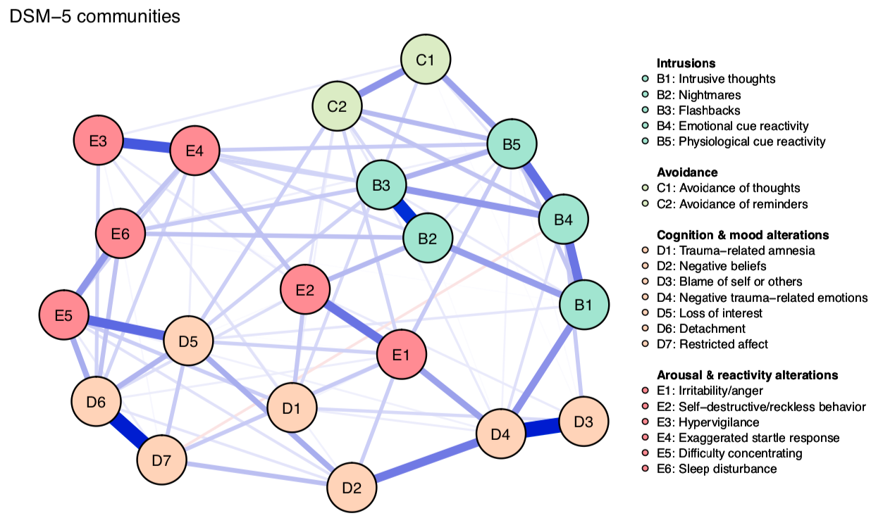
As you can see, the theoretical relations do not seem to map well onto the empirical relations. Especially E2 and E3 do not really closely inter-relate with other nodes from their DSM-5 community.
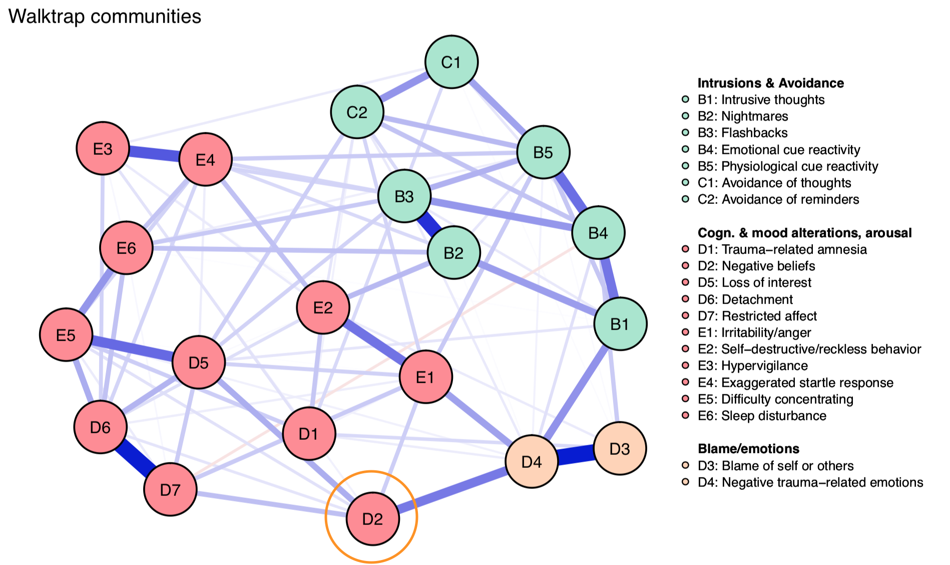
2. PTSD network based on the walktrap algorithm
So let’s estimate the network using the walktrap algorithm, which is implemented in the R package EGAnet:
comm1<- EGA(data, plot.EGA = TRUE); comm1
gr2 <- list('Intrusions & Avoidance'=c(1:7), 'Cogn. & mood alterations, arousal'=c(8,9,12:20), 'Blame/emotions'=c(10:11))

pdf("Network2.pdf", width=8.5, height=5)
g2<-plot(n1, labels=names, vsize=6, cut=0, border.width=1.5, border.color='black', title="Walktrap communities",
          groups=gr2, color=c('#a8e6cf', '#ff8b94', '#ffd3b6'), nodeNames = longnames,legend.cex=.35)
dev.off() |
Walktrap identifies 3 communities:
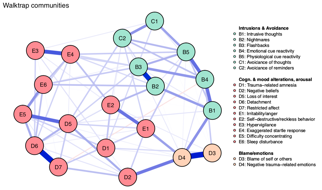
Note that there are several other ways to identify communities, such as spinglass or simply eigenvalue decomposition, which I described in my previous tutorial. I use walktrap here because it’s implemented in EGAnet, and more convenient to estimate.
3. Clique percolation by optimizing I and k
Third, we compare this to the results of clique percolation, for which we use Jens’ CliquePercolation package. You can find more details on the methodology here, which I only summarize briefly. There are several ways of running the algorithm, and I showcase 2 here.
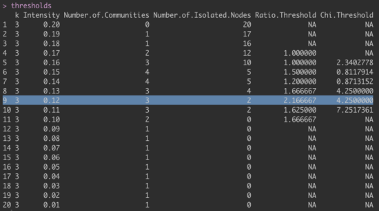
To run the algorithm for weighted networks, one option is to optimize k and I, where I determines how strong the average relations among a community need to be to be detected as a community, and k determines the minimum clique size. CliquePercolation requires a minimum k of 3, so we cannot use k=2, which would have made sense based on the results of the walktrap algorithm that identified a community of 2 nodes (D3 & D4). In the example below, I asked the program to search through ranges of I from 0.01 to 0.20, given that an average partial correlation of 0.20 would appear to be very large. This is usually done for larger networks than we have here, so might not be entirely appropriate.
We then identify the optimal value of I based on the rule that with increasing I, we should extract the solution for which the ratio threshold crosses to values above 2, in the best case accompanied by a large χ value. In our case, this is I=0.12, as you can see in the output below. Missing values (“NA”) are based on the fact that certain metrics can only be computed for networks with at least 2 or 3 communities.
Here the accompanying R code:
### use Clique Percolation
W <- qgraph(n1$graph)

thresholds <- cpThreshold(W, method = "weighted", k.range = 3,
                          I.range = c(seq(0.20, 0.01, by = -0.01)),
                          threshold = c("largest.components.ratio","chi")); thresholds

results <- cpAlgorithm(W, k = 3, method = "weighted", I = 0.12) |
Now we plot the network:
pdf("Network3.pdf", width=8.5, height=5)
g3 <- cpColoredGraph(W, list.of.communities = results$list.of.communities.numbers, layout=L, theme='colorblind',
                     color=c('#a8e6cf', '#ff8b94', '#ffd3b6', '#444444'), labels=names, vsize=6, cut=0, border.width=1.5,
                     border.color='black', nodeNames = longnames,legend.cex=.35,
                     edge.width = 1, title ="PTSD communities based on Clique Percolation")
dev.off() |
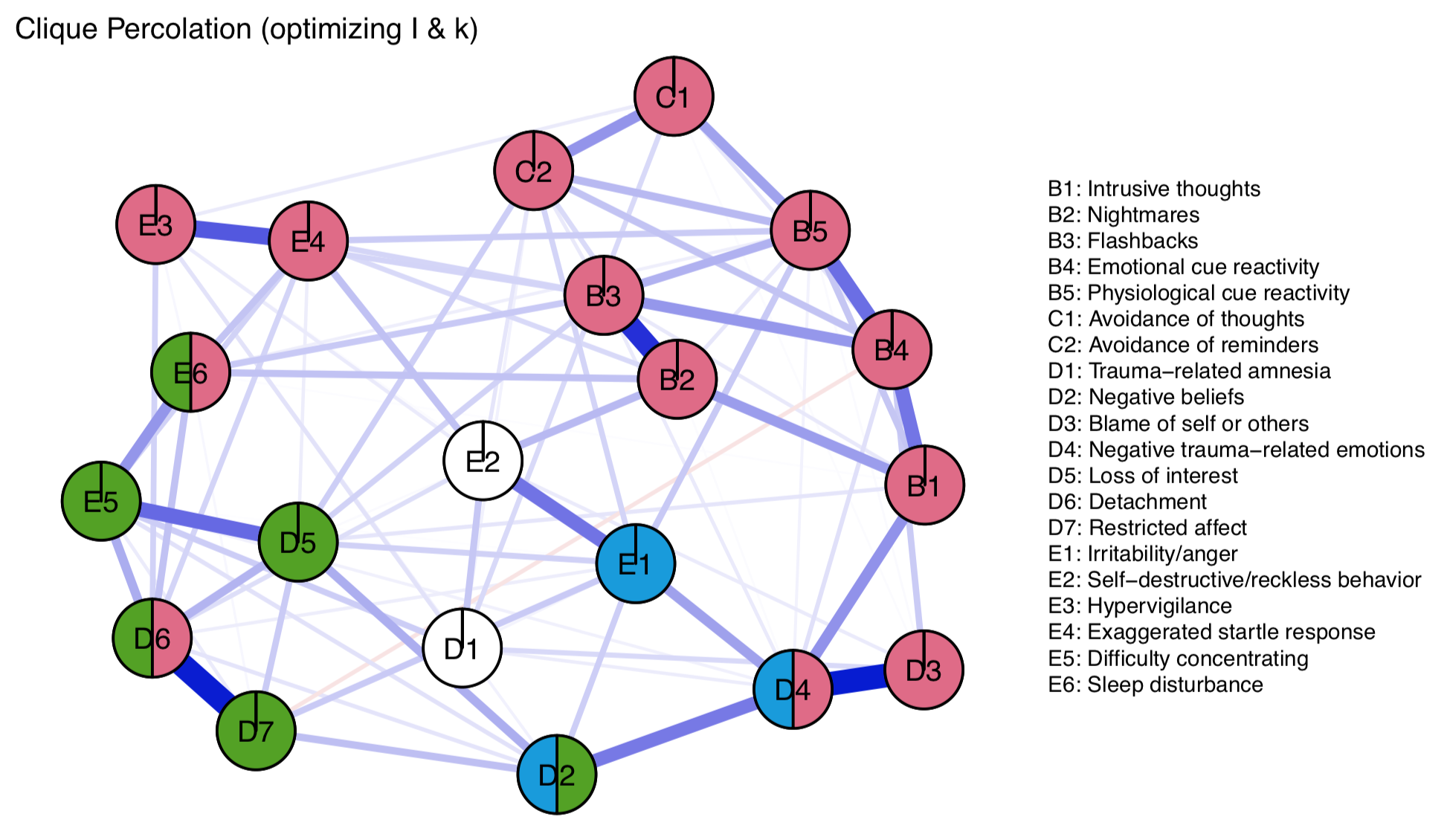
We see that clique percolation also groups a lot of the initial nodes into one group, like the DSM-5 and walktrap; nodes E2 and D1 are not assigned to any community; and 4 nodes are assigned to 2 communities. Overall, results seem sensible, including the assignment of D6 to partially red, given its relations to other red and half-red nodes. Interestingly, E2 is not assigned to any community. Unlike node D1, which has the lowest centrality (i.e. interconnectedness), where no assignment makes sense, E2 is at least moderately connected, to both the blue and red community. EDIT: Turns out we can visualize this via Fruchterman-Reingold easily, so I updated the section above a bit (thanks Jens for your email).
4. Clique percolation by optimizing entropy
A second way that may be better suited for smaller networks is using entropy, based on Shannon information. Jens has a detailed tutorial on that near to the bottom of the package vignette for CliquePercolation, so I will not describe this in detail here. For the PTSD dataset, this method leads us to choose an intensity value of I=0.14 rather than 0.12 above, and the final network solution looks like this:
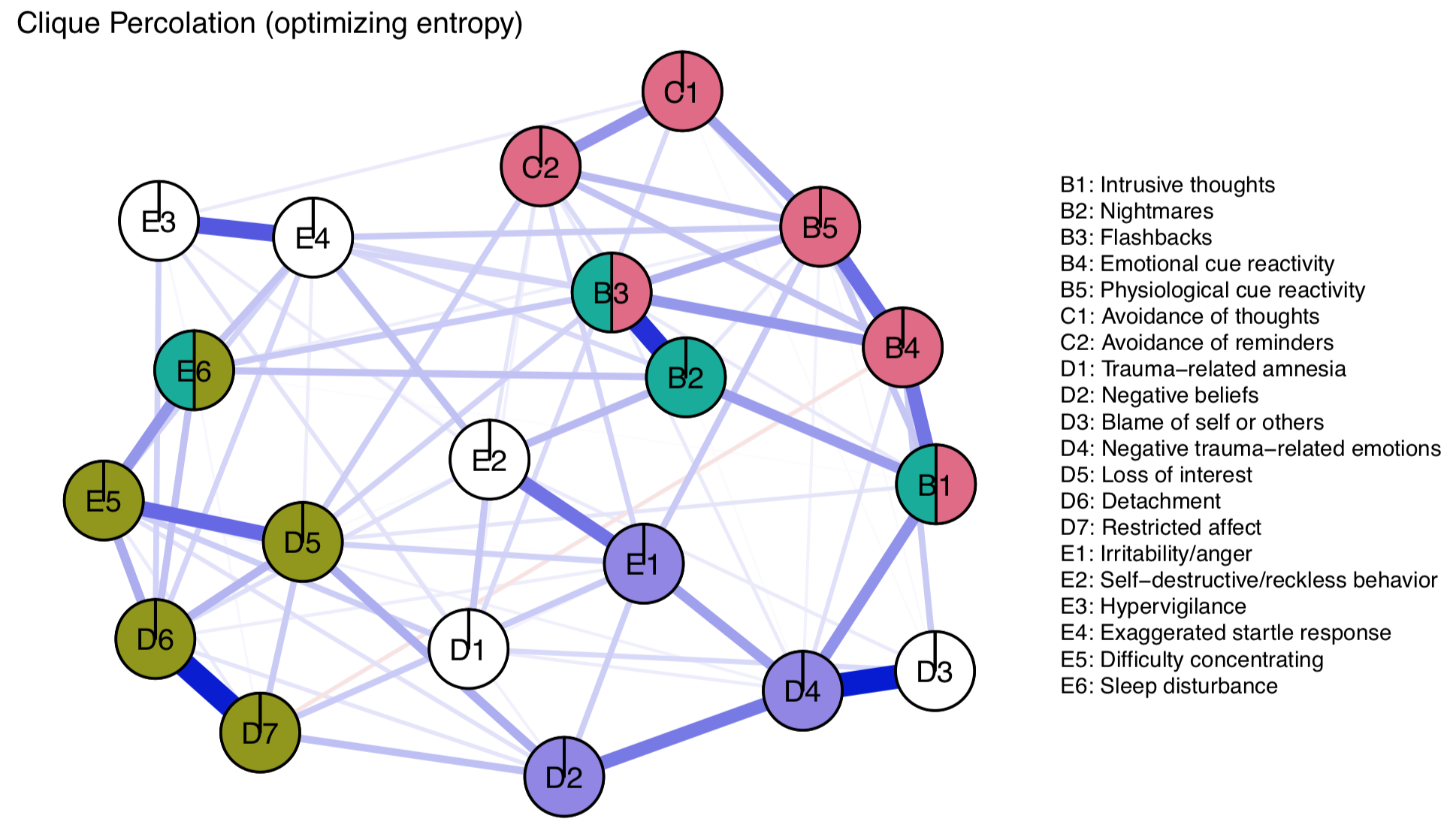
The solution seems overall a bit more conservative, with 5 unassigned nodes. Extracted solutions appear to make sense, although not assigning D3 to a community does not align with prior results, and seems inconsistent given the strong edges the node shows.
Conclusions and ways forward
Data and code for the tutorial are available here. It’s awesome to see commonly used community detection algorithms from other fields being implemented into the free open source software environment, and I see several avenues for future work.
- Model validation: how well does clique percolation recover the true network structure of weighted graphs, under which set of conditions.
- What specific guidelines should we follow to decide what solution to extract? The current guidelines, e.g. for optimizing I and k simultaneously, leave considerable researcher degrees of freedom, which could be exploited if researchers pursue data analysis with certain goals in mind. These lose rules would also make a preregistration of Clique Percolation challenging.
- Power analysis: how many datapoints are required for the method to reliably recover communities, given what specific method?
- Extensions to cases where nodes can belong to more than two communities (akin to cross loadings in the CFA context).
Thanks again Jens for translating cfinder into R3! And if someone finds a way to make the code colorblind friendly (i.e. by assigning different shades/backgrounds to parts of nodes), please do send it over and I am happy to upload it here (with full attribution of course).
- example from here
- Chrome gives me an “unsafe” warning but I have used this resource a lot in the past so I think it should be ok
- Jens let me know that it is not a direct translation, but the method is rather similar; check out the argument method = “weighted.CFinder” for full equivalency
Pingback: Brief psychology news 11/2019 - Eiko Fried
Hi there,
Thank you for the informative tutorial. I’ve been finding it useful as I attempt to apply network analysis to my work with fisheries dynamics. I am very new to network analysis and was wondering if this method of clique percolation can be applied to temporal networks. As a crude analysis I know I could apply this methods to the network at each time step, but I’d like to have the network/community structure of the previous time step inform the network/community structure of the next time step if possible. I really appreciate how this method allows for cross loadings and can’t seem to find a temporal community detection package/method (in R) that allows for cross loadings. Do you know of any packages/methods that utilizes clique percolation in a temporal framework?
Thanks,
Jordan
Community detection algorithms are usually applied to matrices, not data (e.g. spinglass and walktrap in igraph will want a matrix as input). So I don’t see principled concerns to use matrices derived from specific methods. If you use a temporal matrix, e.g. from a VAR model, I would consider omitting autoregressive effects though, given that they really differ from the cross-lagged effects. Or maybe do both, with and without those AR coefficients.
I really enjoyed the tutorial! It actually helped me address some of the comments that the peer reviewers raised about the clustering analysis I used (it was the EGA and they recommended using clique percolation).
The question I have however is – does this method work on networks using binary variables or mixed (binary and ordinal) variables?
All the best!
Marcin
Glad to hear it was useful Marcin!