TL;DR: This blog post summarizes and discusses Information Filtering Networks introduced in a new paper by Christensen et al. 2018, and discusses them compared to the lasso-regularized Markov Random Fields. The post ends with an R tutorial on how to estimate such networks.
Markov Random Fields (MRF) have quickly become the state-of-the-art in psychological network modeling for obtaining between-subjects networks. The implementation for binary data is called the Ising Model, and for continuous or ordinal data, Gaussian Graphical Models (GGMs) have been used1. The beauty of these models is that a zero entry between two variables in the adjacency matrix (i.e. the matrix that encodes the parameters that we then plot as networks) means that the two variables are conditionally independent, given all other variables.
Information Filtering Networks (IFN)
In a new paper entitled “Network Structure of the Wisconsin Schizotypy Scales-Short Forms: Examining Psychometric Network Filtering Approaches”, Christensen et al. (2018)2 introduce Information Filtering Networks (IFNs) to the psychological literature, and compare them to lasso regularized models. Like MRFs, IFNs are partial correlation networks, and the two models differ mainly in one key aspect: addressing a common challenge that Christensen et al. describe very well:
Networks contain multiple connections across all possible pairs of variables (e.g., symptoms, items) included in the model and therefore are likely to have spurious edges (i.e., multiple comparisons problem). Thus, filtering is necessary to minimize spurious connections and to increase the interpretability of the network. This, however, introduces a problem known as sparse structure learning (Zhou, 2011): How best to reduce the complexity and dimensionality of the network while retaining relevant information?
This is a longstanding problem, and many different solutions have been proposed. In MRFs based on lasso regularization, the number of edges is determined largely by fit (i.e. minimizing the extended BIC, see our regularized partial correlation network tutorial). This has a number of advantages: it controls for multiple testing (i.e. for the numerous regressions that the model estimates under the hood); the procedure results in a parsimonious/sparse network structure that is somewhat easier to interpret; and putting coefficients to exact zero means they need not be estimated anymore, which reduces the number of parameters. The default lasso procedure sacrifices specificity for sensitivity, meaning that edges in the estimated network are also very likely in the data, but that some (weak) edges in the data might not be recovered by the lasso.
Lasso criticism
Christensen et al. consider the lasso as “biased” because edges included in MRFs are a function of sample size. I wouldn’t call this a bias, but it is correct that the lasso puts even moderately large edges to zero in situations of low power because it cannot reliably distinguish these edges from zero, whereas the lasso will put nearly no edges to zero in extremely large samples because it can very reliably distinguish even tiny edges from zero3. I think about the lasso as a feature that works very similar in standard statistical methods used in psychological research: if a correlation of 0.2 is estimated in a small sample with little power, its confidence intervals (CIs) are large and often overlap with 0 [CI -0.6; 0.8]. In this case, we treat the coefficient as not significantly different from zero. But if we have sufficient power, a correlation coefficient of 0.2 might well be distinguishable from zero [CI 0.1;0.3].
How do IFNs determine the number of edges?
How are edges chosen in the IFNs, if not based on the lasso? The paper by Barfuss et al. 20164 provides a fantastic introduction to IFNs, and also covers the lasso, ridge regression, and the elastic net.
IFNs deal with the issue of minimizing spurious relations not by choosing the edges based on fit to the data. Instead, IFNs estimate a fixed number of edges based on the formula “3 * nodes – 6”. A network with 20 nodes has 54 (out of 190; ~28%) edges, and the networks the authors estimate in the paper, with 60 nodes, have 174 (out of 1770 potential; ~10%) edges. I see two main challenges here.
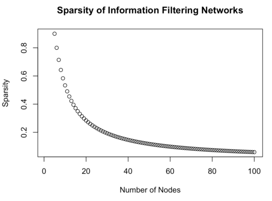
First, in case two networks differ from each other (i.e. one has many connections, the other fewer), estimating the same number of edges in both networks might artificially inflate similarity between the structures—or it might lead to the opposite. Without simulation studies, which the paper does not contain, we do not know, and conclusions are premature. Second, I could find no rationale why “3 * nodes – 6” would be a reasonable formula for the number of edges we expect in psychological network structures. There might be some general rules that emerge across psychological networks, and maybe it turns out to be a good approximation. But it seems a strong assumption to me. The procedure is similar to running a linear regression with 10 predictors and determining before looking at your data that 3 will be different from 0. It is also worth noting that IFNs get sparser with a larger number of nodes: with k=10 nodes, 24 of 45 edges are estimated (nearly 50%), but in k=100, 294 of 4950 edges are estimated (6%).
Below a visualization of the relationship between the number of nodes, and the sparsity (i.e. % of estimated IFN edges in relation to all potential edges):
matrix <- matrix(NA, nrow=2, ncol=100)

for (n in 5:100) {
matrix[1, n] <- n*3-6      #edges in IFN
matrix[2, n] <- n*(n-1)/2  #all potential edges in network
  }

plot(matrix[1, ] / matrix[2, ], ylab="Sparsity", xlab="Number of Nodes", main="Sparsity of Information Filtering Networks") |

This behavior serves the goal to estimate sparse network structures. But it’s also easy to think of scenarios in which IFNs will do a bad job at recovering the true network structure. For instance, imagine a scenario where the true network structure has many nodes and is dense: the IFN will always lead to a very sparse network. Then again, we can envisions scenarios as well where the lasso would not perform well, such as a dense true structured estimated in a small sample.
Disagreements
There are some statements in the paper I disagree with, and I post them here as post-publication review in the hopes that it will lead to a dialogue with the authors so we can resolve potential misunderstandings together.
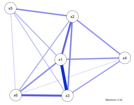
First, Christensen et al. write that in a case of a lot of shared variance among items, the focus of MRFs on unique variances will remove the shared variances, leaving items disconnected5. They reference the paper of Forbes et al. 2017 discussed previously that was written under the same assumption. But the opposite is the case: if all items share a lot of variance, i.e. if a unidimensional factor model describes the data well, the network will be fully connected. In other words, if you simulate data from a unidimensional factor model, you get a fully connected, not an empty network model; this has been shown many times both in simulation studies and in mathematical proofs. See below where we first simulate data (n=300) from a unidimensional factor model, and then fit a MRF to the data that is fully connected, resulting in considerable partial correlations (all code available here).
# Lavaan simulation population.model <- ' f1 =~ x1 + 0.8*x2 + 1.2*x3 + 0.7*x4 + 0.5*x5 + 0.8*x6' set.seed(1337) myData <- simulateData(population.model, sample.nobs=300L) fitted(sem(population.model)) round(cov(myData), 3) round(colMeans(myData), 3) myModel <- ' f1 =~ x1 + x2 + x3 + x4 + x5 + x6' fit <- sem(myModel, data=myData) summary(fit) network2 <- estimateNetwork(myData, default="EBICglasso") plot(network2, details=TRUE) |

Second, the authors state that “The shrinkage of correlations below a certain threshold [when using the lasso] also contributes to reduced reproducibility because variables can be eliminated based on statistical significance rather than theory.” The lasso does not eliminate variables, it eliminates edges. The goal is to estimate a model that describes the data well, whilst avoiding the estimation of spurious relations by finding a good balance between false positive and false negatives. IFNs do the same: they are data-driven models that differ from MRFs in that they use a different strategy to obtain a parsimonious structure. So if there is any criticism regarding theory (which is an argument one can make), it applies to both models.
Third, the authors conclude that the pitfalls of the lasso-based MRFs are “biased comparability, reduced reproducibility, and the elimination of hierarchical information”. With biased comparability they mean that the lasso regularizes proportional to power, which is true: if we simulate data for n=200 and n=2000, both times from the same true network structure, and estimate networks for both datasets, the network in n=200 will likely be sparser than the network in n=2000 (i.e. fewer edges), because that is how the lasso operates. It has more power in n=2000 to reliably distinguish small edges from zero, similar to t-tests or linear regressions that can more reliably detect differences (e.g. from zero) in larger samples. But this also means that this main criticism can simply be circumvented by either a) making sure sample size is similar when comparing network structures, which is commonly done6, or b) by using permutation tests that take sample size into account when comparing network structures, which the Network Comparison Test developed exactly for this purpose does. The second point “reduced reproducibility”, is primarily based on assertions of Forbes et al. 2017, all of which have been thoroughly refuted7. Christensen et al. add to the argument by comparing 2 network structures of 2 datasets, and find that IFNs have higher replicability than MRFs8. Even if we, for the sake of the argument, do not object to the way Christensen et al. conduct the comparison, the conclusion that IFNs replicate better in this specific case allows no conclusion whatsoever about replicability of models in general. And obviously, the authors retrieve the same amounumbert of edges across the two network structures because IFNs a priori estimate the same number of edges in case the number of nodes is the same. For their last point, “elimination of hierarchical information”, I do not understand how IFNs get around that.
Finally, it is odd to read Christensen et al.’s repeated criticism of partial correlations and conditional dependence relations … given that the network model they put forward is a partial correlation network / conditional independence network.
In general, what I would have loved to see in the paper is a simulation study that actually shows how IFNs perform, which is necessary to vet any proposed methodology. That is, it is crucial to show that if you simulate data from a known structure X, your methodology will do well in recovering that structure.
R tutorial
I’m extremely thankful Christensen et al. 2018 brought IFNs to the world of psychological network modeling. From my perspective, we have two different approaches, and it is premature to conclude that one approach is inherently superior to the other; this goes both ways, obviously. The benefits likely depend on the context, such as the true network structure the data come from, prior knowledge about the network structure, the sample size, and the number of nodes.
Sacha Epskamp, who programs faster than light, has implemented IFNs in our R-package bootnet and sent around example code I will paste below. This was possible because Christensen et al. implemented the estimation routine in the package NetworkToolbox.
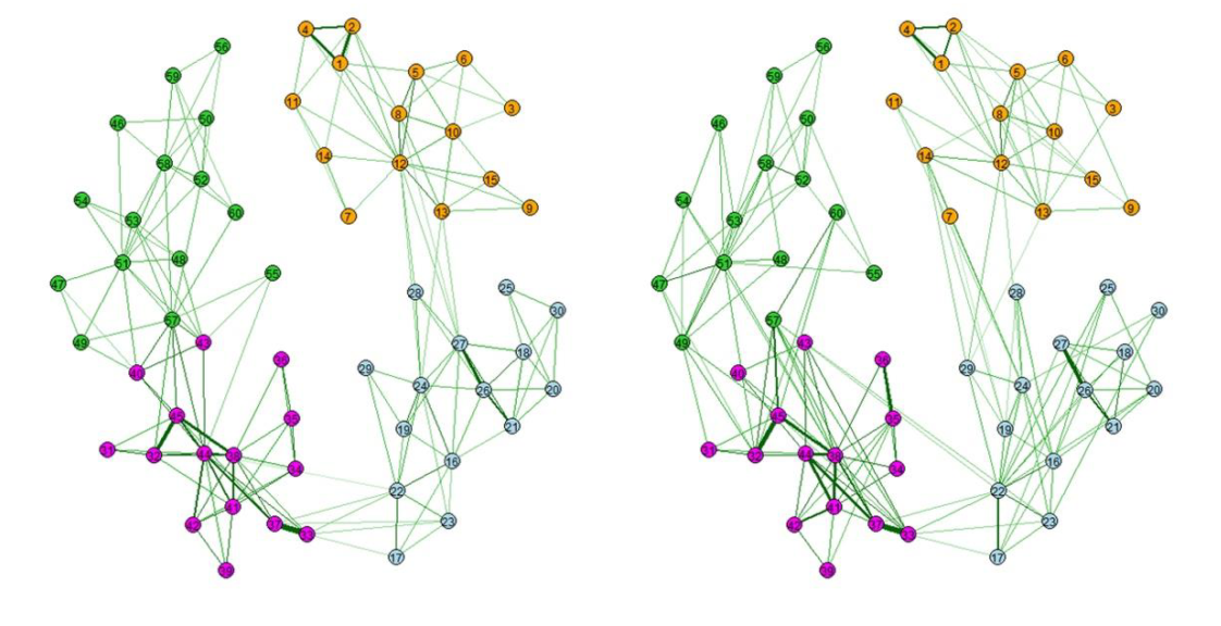
You can estimate the models via estimateNetwork(default="TMFG"). The below code estimates a MRF and a IFN on the same data, and compares them superficially. As dataset we use the BFI data that are openly available.
# Install packages:
devtools::install_github("sachaepskamp/bootnet")
library("NetworkToolBox")
library("bootnet")
library("psych")
library("qgraph")

# Estimate networks, first a Gaussian Graphical Model, then an Information Filtering Network:
data(bfi)
LassoNetwork <- estimateNetwork(bfi[,1:25], default = "EBICglasso")
TMFGNetwork <- estimateNetwork(bfi[,1:25], default = "TMFG")

# Average Layout so networks can be compared:
Layout <- averageLayout(LassoNetwork, TMFGNetwork)

# Plot both networks using the same layout:
layout(t(1:2))
plot(LassoNetwork, layout = Layout, title = "EBIC glasso")
plot(TMFGNetwork, layout = Layout, title = "Triangulated Maximally Filtered Graph") |
IFN stability
I’ve worked a lot on stability of network models in recent years, together with Sacha Epskamp, and a natural question that follows this work is: how stable are IFNs, and how stable are they compared to MRFs?
One quick look in one dataset — obviously, this does not generalize to anything but this specific dataset — leads to fairly low stability in some edges, but excellent stability in others, which is not surprising. Imagine you have 20 nodes in a network, with 30 strong edges, 30 moderate edges, 30 weak edges, and 100 absent edges. The IFN will always estimate 20*3-6 = 54 edges. This means it will correctly estimate the 30 strong edges, but then pick 24 of the 30 equally strong moderate edges. Every time you bootstrap the network, you will pick a random selection of 24 moderately strong edges. Overall, the estimation of the very strong and very weak edges will be stable (i.e. always very similar when bootstrapping), but moderately strong edges will be estimated with low precision.
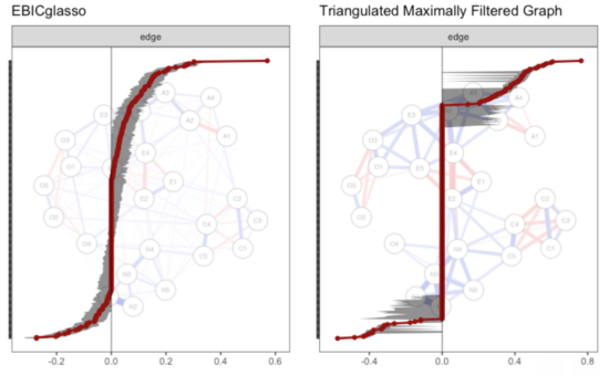
Estimating and bootstrapping MRF vs IFN using the BFI dataset leads to the following edge weights and CIs (again, codes & graph from Sacha)9:
boot1lasso <- bootnet(LassoNetwork, nBoots =1000, nCores = 8) boot1tmfg <- bootnet(TMFGNetwork, nBoots =1000, nCores = 8) plot(boot1lasso, labels = FALSE, order = "sample") plot(boot1tmfg, labels = FALSE, order = "sample") |

So there is plenty of future work to do, and I hope the next paper on IFNs will contain some simulation studies to vet their performance in different situations.
Acknowledgements
We discussed the paper in the labgroup, and the blog post is a summary of many points raised there. Obviously, all mistakes in the blog post are my mistakes only.
Footnotes
- The GGM has been largely used for estimating between-subjects networks in cross-sectional data, but has recently been extended and integrated into time-series models.
- Christensen, A. P., Kenett, Y. N., Aste, T., Silvia, P. J., & Kwapil, T. R. (2018). Network Structure of the Wisconsin Schizotypy Scales-Short Forms: Examining Psychometric Network Filtering Approaches. Behavior Research Methods. http://doi.org/10.3758/s13428-018-1032-9.
- For a paper describing this behavior in more detail, see: Epskamp, S., Kruis, J., & Marsman, M. (2016). Estimating psychopathological networks: be careful what you wish for. arXiv: 1604.08045.
- Barfuss, W., Massara, G. P., Di Matteo, T., & Aste, T. (2016). Parsimonious modeling with information filtering networks. Physical Review E, 94(6), 1–12. http://doi.org/10.1103/PhysRevE.94.062306
- Quote: “Because each symptom is regressed over all others, it’s likely that the shared variance between these high scores will be removed, thereby leaving some symptoms completely disconnected.”
- For instance, in these two papers: Fried, E. I., Eidhof, M. B., Palic, S., Costantini, G., Dijk, H. M. H., Bockting, C. L. H., … Karstoft, K. (2018). Replicability and Generalizability of Posttraumatic Stress Disorder (PTSD) Networks: A Cross-Cultural Multisite Study of PTSD Symptoms in Four Trauma Patient Samples. Clinical Psychological Science. http://doi.org/10.1177/2167702617745092; Rhemtulla, M., Fried, E. I., Aggen, S. H., Tuerlinckx, F., Kendler, K. S., & Borsboom, D. (2016). Network analysis of substance abuse and dependence symptoms. Drug and Alcohol Dependence, 161, 230–237. http://doi.org/10.1016/j.drugalcdep.2016.02.005.
- Further reading: https://psych-networks.com/network-models-do-not-replicate-not/
- I use the term replicability here, because my definition of reproducibility is whether you can obtain the same result using the same dataset & methodology.
- The graphs look different from what you get, but I want to keep the codes simple here.

Pingback: Looking back at 2018 - Eiko Fried