Lizanne Schweren, a Postdoc at the University Medical Center Groningen, and colleagues published a paper in JAMA Psychiatry this morning showing that the connectivity of depression symptoms is, in contrast to what a prior paper found, not a predictor of treatment response. This is the first non-replication in the psychopathology network literature I’m aware of1.
The blog is structured into 5 sections:
- I will describe the original paper by van Borkulo et al. 2015
- Explain what network connectivity is which both teams investigated
- Show, in a reproducible R-tutorial with data and code, how to compare connectivity across networks
- Present the results of the new paper by Schweren et al. 2017
- And end with a call for a multi-sample high-powered replication of this effect, and add some further considerations.
Then I’ll eat breakfast.
Van Borkulo et al. 2015
Back in 2015, Claudia van Borkulo, a postdoc in the Psychosystems Group in Amsterdam, and colleagues published a paper entitled “Association of Symptom Network Structure With the Course of Depression” in JAMA Psychiatry2 that has gathered nearly 80 citations since3.
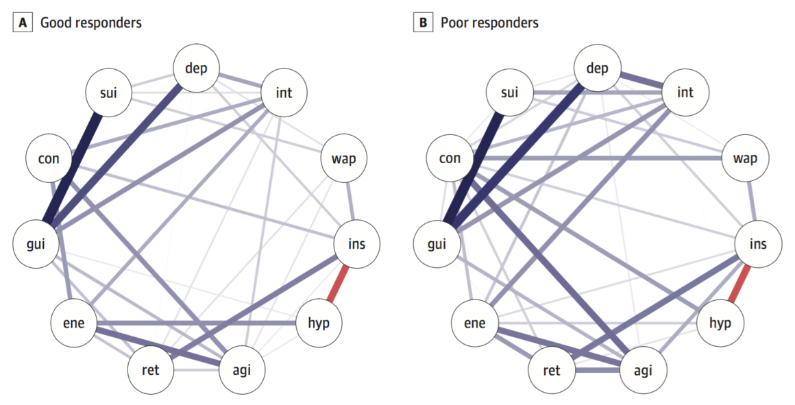
In the paper, the authors took 515 participants from the NESDA cohort with last-year diagnosis of MDD, and split the sample into two groups at the follow-up timepoint 2 years later: treatment responders vs treatment non-responders. Van Borkulo et al. then estimated network structures at timepoint 1 for these two groups, and found that the non-responder group at baseline had higher network connectivity than the responders, i.e. the absolute sum of all edges in the network structure.
The test statistic for the difference in network connectivity was 1.79 (p = .01). In two sensitivity analyses, the test statistic remained significant (analysis 1: 1.55, p = .04; analysis 2: 1.65, p = .02).
Connectivity
So what is global connectivity or global density, and why might it be relevant? Connectivity is the sum of all the things going on in a network structure, and it depends on what kind of network you have to make sense of it. In a temporal network collected with time-series data, for instance, you could add all temporal cross-lagged effects per patient (sad mood predicting anhedonia; concentration problems predicting sleep problems; etc.), and then see if there is more going on for patient A than B. You could add to that the autoregressive coefficients (sad mood on sad mood; anhedonia on anhedonia), and then you’d have a measure of temporal density. You could interpret this of sum of “activation” carried from one time-point to the next, and compute some kind of R^2 (if the temporal connectivity is 0, then you also explain no variance of one timepoint to the next).
In cross-sectional between-subjects networks, connectivity is simply a sum of all absolute edge values4. It means that, in a given population, items tend to have stronger conditional dependence relations, which usually also means items have higher correlations; in a factor model perspective, this can translate into higher Cronbach’s Alpha, i.e. scale reliability.
How do you compute global density? You can download a freely available example dataset here, including code5.
library("qgraph")
library("bootnet")
load("data.Rda")
network1 <- estimateNetwork(data, default="EBICglasso", corMethod="cor")
graph1 <- plot(network1, layout="spring", cut=0)
sum(abs(network1$graph))/2

#global density: 8.48 |
We load the data, estimate a network, plot the network (not shown), and then compute connectivity. We have to divide the absolute sum by 2 because all edges are encoded twice in the adjacency matrix (A with B but also B with A).
Network Comparison
How do you compare global connectivity across two networks? Claudia van Borkulo developed the Network Comparison Test (NCT) for that purpose.
First, let’s split our data into two sub-datasets that we want to compare.
library("dplyr")
data1 <- slice(data, c(1:110))
data2 <- slice(data, c(111:221)) |
We then estimate and plot two network structures:
network2 <- estimateNetwork(data1, default="EBICglasso", corMethod="cor") network3 <- estimateNetwork(data2, default="EBICglasso", corMethod="cor") graph2 <- plot(network2, layout="spring", cut=0, details=T) graph3 <- plot(network3, layout="spring", cut=0, details=T) L <- averageLayout(graph2,graph3) layout(t(1:2)) graph2 <- plot(network2, layout=L, cut=0, maximum=0.29) graph3 <- plot(network3, layout=L, cut=0, maximum=0.29) |
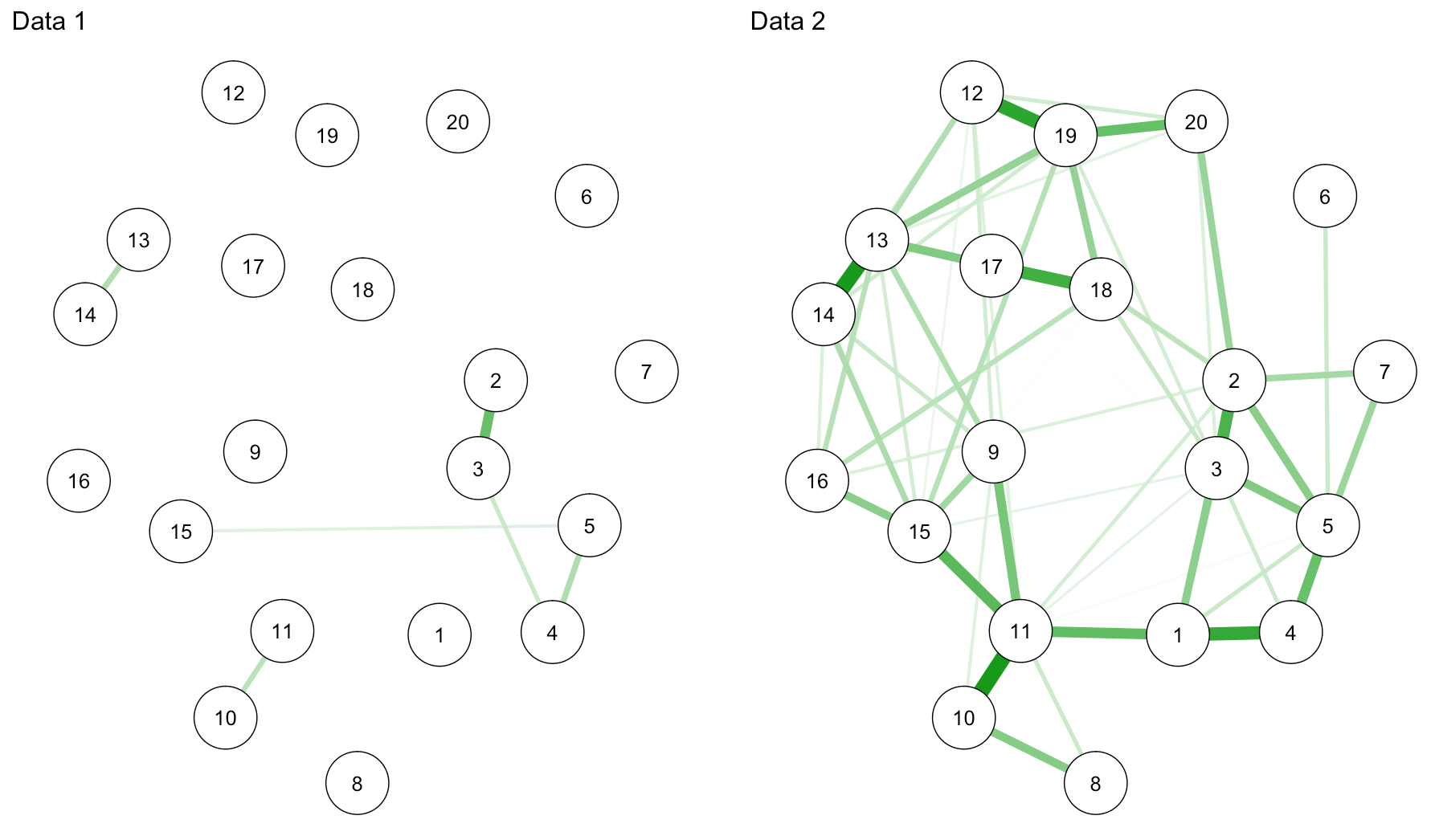
Haha … I swear I only split the data once (back in summer this year! for a workshop in Spain), so for this tutorial, from an educational perspective, I guess we’re lucky we get so pronounced connectivity differences.
sum(abs(network2$graph))/2 #0.5436501 sum(abs(network3$graph))/2 #5.794574 |
Now, on to the NCT, a permutation test that tests against the null-hypothesis that networks have identical connectivity:
nct_results <- NCT(data1, data2, it=1000, binary.data=FALSE) |
This gives us 3 main outcomes:
nct_results$glstrinv.sep # connectivity values: 0.54 vs 5.79 nct_results$glstrinv.real # difference in connectivity: 5.25 nct_results$glstrinv.pval # global strength invariance: 0.71 |
The first line replicates connectivity that we estimated by hand above; the second lists the difference that was used as test statistic in the permutation test; followed by the p-value.
We now have a perfect example showing that the NCT requires sufficient power to detect differences between the connectivity of two networks — because networks that do seem to differ in connectivity (both graphically and statistically), as in the example above, are found to be identical in connectivity due to the small sample size here (Claudia shows this clearly in her NCT validation paper that is, I believe, still under revision). So if the NCT is non-significant, and you have two small samples, this can mean that there is no difference, or that there is not enough power to detect the difference. This is important to keep in mind.
(Note that you can compare networks in many more ways than just connectivity. The Network Comparison Test can also test for differences in network structure, and differences in all individual edges; further, there are other tests available such as assessing the similarity of network structures. For 2 example papers where we did all of this, including all code how to do it, see 1 and 2.)
Schweren et al. 2017
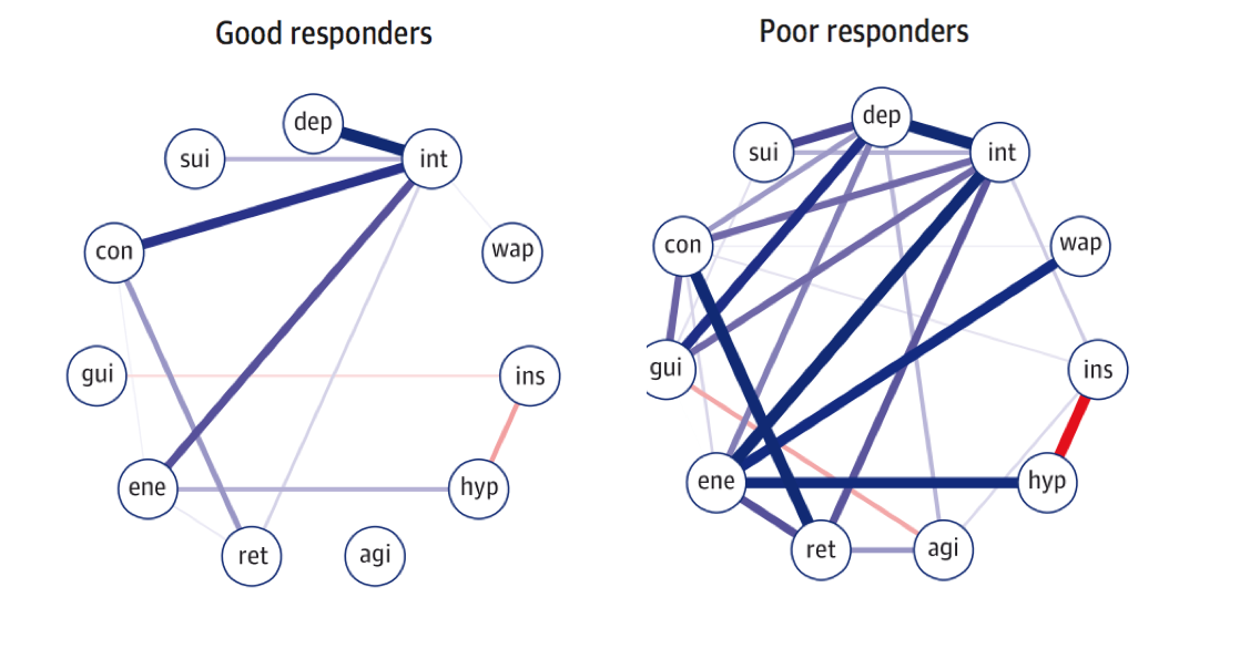
On to the new paper by Schweren et al. 2017 that was a conceptual replication of van Borkulo et al. 2015. We also split the data based on timepoint 2 into responders and nonresponders, but the baseline networks for these two groups do not differ in connectivity:

Global connectivity was higher in poor responders, similar to the paper by van Borkulo et al., but the difference was not significant (good responders, 3.6; poor, 4.3; p = 0.15).
Lesson learned?
It’s very cool to see critical replications and non-replications, and I think we should do that much more for substantive findings that might be relevant. For this particular effect, I am still not convinced what to think, given the fact that the result went into the same direction, and the connectivity difference between networks wasn’t negligible.
How about we write a high-powered follow-up study with multiple larger samples? I have the STAR*D data lying around (~3500 patients) I could contribute, if anybody is interested to replicate this with higher power: let me know, let’s join up, let’s do it. Code from two papers, expertise, and plenty of co-authors interested in this are available! And I’m sure I’m not saying too much if I include Claudia and Lizanne here as potentially interested candidates for collaborations ;)!
Complications
One fairly severe complication is that in the tutorial above, I used CorMethod=”cor” when estimating networks for simplicity, which forces estimateNetwork() to use Pearson instead of polychoric correlations for the skewed ordinal items in the data (these are PTSD symptoms in a subclinical sample, so substantial skew). This is, of course, inappropriate. If I repeat the analysis with polychoric correlations, the connectivity for the networks is 8.30 vs. 8.38, very much identical (compared to 0.54 vs 5.79 that we got from the Pearson correlations, a pronounced difference). The strongest edge is now 0.48 instead of 0.28.

The results change dramatically, which implies the importance of looking at the distribution and type of your data, and make sure you use the appropriate correlations. Sacha Epskamp and I describe this in some detail in the FAQ of our new tutorial paper on regularized partial correlations forthcoming in Psychological Methods.
Further confusions
There is considerable evidence, across numerous datasets I reviewed in a recent empirical, and also in two very large datasets I studied for that paper, that network structures of depression symptoms in healthy people are more highly interconnected that network structures of depression symptoms in depressed people6. Many explanations have been offered for this, and although I’ve worked on this for over 3 years now, I really haven’t figured out how to make sense of these findings, or how to make sense of them in relation to the findings by Claudia and Lizanne. If you’re interested (or have suggestions to offer), I summarized the paper in this blog post.
And now:

Footnotes:
- Not because all other results replicated, but because so far work has been largely exploratory and there are none to very few (depending on where you stand) real ‘findings’ except for “this is the network structure in dataset X”; but it’s early and I haven’t had breakfast, so I might have my grumpy hat on and regret writing this after my first coffee.
- van Borkulo, C. D., Boschloo, L., Borsboom, D., Penninx, B. W. J. H., Waldorp, L. J., & Schoevers, R. A. (2015). Association of Symptom Network Structure With the Course of Longitudinal Depression. JAMA Psychiatry, 72(12), 1219. http://doi.org/10.1001/jamapsychiatry.2015.2079
- This is pretty much the number of all network papers since, so it’s an incredibly well-cited paper.
- Absolute because arguably, negative edges still add up to connectivity; this is debated, however, cf. Robinaugh, D. J., Millner, A. J., & McNally, R. J. (2016). Identifying highly influential nodes in the complicated grief network. Journal of Abnormal Psychology, 125(6), 747–757. http://doi.org/10.1037/abn0000181
- From: Armour, C., Fried, E. I., Deserno, M. K., Tsai, J., & Pietrzak, R. H. (2017). A network analysis of DSM-5 posttraumatic stress disorder symptoms and correlates in U.S. military veterans. Journal of Anxiety Disorders, 45. http://doi.org/10.1016/j.janxdis.2016.11.008.
- Fried, E. I., van Borkulo, C. D., Epskamp, S., Schoevers, R. A., Tuerlinckx, F., & Borsboom, D. (2016). Measuring Depression Over Time … or not? Lack of Unidimensionality and Longitudinal Measurement Invariance in Four Common Rating Scales of Depression. Psychological Assessment, 28(11), 1354–1367. http://doi.org/10.1037/pas0000275
Pingback: A Network Analysis Replication: OCD & Depression Comorbidity – Payton J. Jones
Pingback: 6 new papers on network replicability | Psych Networks
Thank you for this tutorial and for sharing your impressive work online!
I’d like to perform a Network Comparison Test on a dataset consisting mostly of mixed ordinal data, but with a few continuous variables. Would this be a problem? Which type of estimator should I use? Thanks for any help you can give.
Best,
Ale
Hi Ale, to my knowledge the NCT is implemented only for Gaussian Graphical Models and Ising Models, but not Mixed Graphical Models.
Hello Eiko,
Thank you so much for your brilliant posts! As a student who is a complete newbie in network science, I’ve found them incredibly useful! I’m wondering if you have any advice about how one can compare multiple networks (in my case three) in terms of global strength and connectivity. I understand that the Network comparison test as implemented in R can be used to compare two networks at a time. Would it be feasible to compare the outputs from a pairwise comparison and apply and multiple comparison corrections? Or perhaps there is a better way to achieve this. Any advice, links, reading would be much appreciated!
Hi Sylvie, thanks for the kind words. We had the same question for a paper that was published very recently, where we wanted to compare 4 networks. We went for pairwise comparisons without correction for multiple testing for the NCT, accompanied by correlating adjacency matrices and centrality rank order. Combined, we believe that these metrics provide a fuller picture.
You can find the paper here. Supplementary materials contain a) all code on how to do all of this, and b) the correlation matrices of the data so you can fully reproduce the main analyses.
http://journals.sagepub.com/doi/abs/10.1177/2167702617745092
Cheers
Eiko
Thank you so much. This was very useful!
Hello Eiko,
Thank you for sharing your excellent work! As a newbie, I have learned a lot from your blog. It inspired me a lot!
I am working on a network comparison using Network Comparison Test and I am confused at one point after reading this blog. In the “Complications” part, you mentioned that if polychoric correlations were used instead of CorMethod =” cor” when estimating networks, the connectivity for the networks will change to 8.30 vs. 8.38. But you didn’t suggest how to compare these two new networks in this situation. I observed that only original data sets were used in Network Comparison Test, i.e. NCT(data1, data2, it=1000, binary.data=FALSE).
I am wondering whether the methods or correlations used in network estimating will change the results of NCT? For example, whether there are differences in NCT if the networks were estimated using CorMethod=” cor” or CorMethod=” spearman”? Any advice would be appreciated!
It’s been a while since I looked into the NCT literature. The original NCT paper by Claudia van Borkulo was available only as preprint for the longest time, so I’d check if that’s published. In that paper, the NCT was only validated for Pearson correlations. That means the sim studies and thresholds are for networks of normally distributed variables where the variance/covariance matrix which networks are constructed upon is estimated via Pearson correlations.
Anything else is easily possible to do, by exchanging the correlation function in NCT, but it’s important to note this isn’t validated.
“I am wondering whether the methods or correlations used in network estimating will change the results of NCT?”
That depends. If your data are normal, it probably doesn’t matter if you use Pearson or Spearman or polychorics (the latter only with sufficient observations, otherwise you can run into issues). If data are heavily skewed or something similar, Pearson is not appropriate, and changing to e.g. Spearman will change your correlation matrices, and, correspondingly, your networks, which can affect the NCT results of course.
Appreciate your quick response! I can imagine that the change of correlation matrices can affect the NCT results accordingly, But I didn’t observe any arguments involved in correlation methods in NCT, listed as follows:
NCT (data1, data2, gamma, it = 100, binary.data=FALSE, paired=FALSE, weighted=TRUE, AND=TRUE, abs=TRUE, test.edges=FALSE, edges=”all”, progressbar=TRUE, make.positive.definite=TRUE, p.adjust.methods= c(“none”,”holm”,”hochberg”,”hommel”,
“bonferroni”,”BH”,”BY”,”fdr”), test.centrality=FALSE, centrality=c(“strength”,”expectedInfluence”),nodes=”all”, communities=NULL,useCommunities=”all”, estimator, estimatorArgs = list(), verbose = TRUE)
Do you have any idea about it?
“In that paper, the NCT was only validated for Pearson correlations. ”
I think you are right, I read that paper. I estimated networks using Spearman correlation and have no idea how to do the network comparisons. But I observed someone else do this using NCT, the author of the following paper estimated networks using partial Spearman correlations and did the NCT, which confused me further.
https://journals.sagepub.com/doi/abs/10.1177/10731911211050921
There are forks of NCT on Github (I believe by Sacha Epskamp, also Payton Jones I think) that allow you to install NCT and then use e.g. polychoric or Spearman, I believe. So just google NCT Github and these names and you should find it. Maybe there are also easier ways to do that using NCT itself but I wouldn’t know—worth asking the maintainer (Claudia van Borkulo). Or just post the question in our “psychological dynamics” facebook group where the authors answer questions like that.
Thanks a lot for sharing this!