Bootstrapping edges after regularization: clarifications & tutorial

I have read the following statement numerous times in the last months: “If the 95% boostrapped CI of an edge weight in a network contains zero, the edge cannot be differentiated from zero”. This is incorrect in case of regularized partial correlation networks, and I thought I would write this up as a short public answer I can refer to more easily in the future.

One of the core features of the R package bootnet is bootstrapping of network edge weights. Bootstrapping is a procedure where you estimate your network structure and parameters of interest many times (e.g. 1000), each time with a slightly different sample. You obtain these different samples by drawing people from your data randomly with replacement. This means that in your first bootstrap, Bob might be in there 3 times (but not Alice), whereas in the second bootstrap, Alice is in there twice (but Bob is absent). The larger the sample, and the more similar the people to each other, the more stable your parameters will be.

We put together bootnet to give you an idea about the stability of the edge weights and other parameters. If the edge between two nodes, A and B, is widely different every time you resample, it means your bootstrapped 95% CI will be all over the place. I have described bootnet and its functionalities in a previous tutorial blog post, and we have a tutorial paper on bootnet that was published in 2017.

Here, for instance, is the output of the bootnet() function in bootnet from our recent CPS paper for dataset 1, available in the supplementary materials:

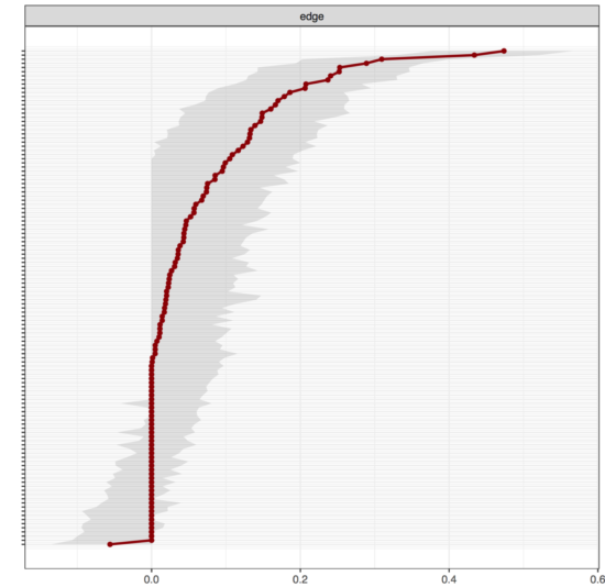
On the y-axis are all 120 edges in the network (labels omitted to keep it legible), the x-axis shows the strength of the edge weights (you can see that nearly all edge weights are positive). The red dots are the point estimates of all edges, the grey area the “95% bootstrapped CI”, as I used to call it. The important point is that many of the CIs will just overlap with zero. How do we interpret this? Usually, if a point estimate of a parameter is 0.1 (e.g. a correlation), we do not know if that parameter is different from zero. This is a normal situation in statistics, and the reason why we usually look at the CI coverage: if the CI includes 0, the parameter cannot be differentiated from 0.

In the case of regularized partial correlation networks, the story is different. If an edge is 0.1 after regularization, that means we have two types of information about the parameter: 1) our best guess is that the parameter is 0.1; 2) our best guess is that the parameter is different from 0.

Why? because we use regularization, a well-validated, sophisticated statistical technique to only keep coefficients in the network that are not zero¹. Obviously, regularization can still lead to errors, there are situations in which regularization does not do well, and there are numerous other methods that should be considered when estimating networks (for a summary on these points, see Sacha Epskamp’s recent blog post). But the main point is that we have to interpret the 95% CI of regularized edge weights differently than we usually do.

For the supplementary materials of a network paper on depression symptoms & inflammation that we are about to submit, Jonas Haslbecks helped us look at this topic from a somewhat different angle, and also provided some insights on the topic. It would take me more sentences to reiterate what Jonas said very concisely, so I will simply paste the relevant part of the supplementary materials here:

“In order to quantify the uncertainty associated with all edge-estimates, we computed a bootstrapped sampling distribution based on 100 bootstrap samples, for each of the edge-estimates. For each of the six networks estimated in the main article we present summaries of the p(p-1)/2 bootstrapped sampling distributions, one for each edge parameter. Specifically, we display the 5% and 95% quantiles of the bootstrapped sampling distribution and show the proportion of nonzero estimates on point that indicates the mean of the sampling distribution.
Because we use regularization to estimate the network models, all edge-estimates are biased towards zero, which implies that all sampling distributions are biased towards zero. Thus, these sampling distributions are not Confidence Intervals (CIs) centered on the true (unbiased) parameter value. This means that if the quantiles of the bootstrapped sampling distribution overlap with zero it could be that the corresponding CI does not overlap with zero. However, if the quantiles of the bootstrapped sampling distribution do not overlap with zero, we know that also the corresponding CI does not overlap with zero (explained in detail in Epskamp, Borsboom & Fried, 2017). Further details of bootstrap analyses are available in the supplemented R code.”

Jonas also produced the following plot²:

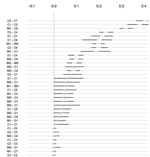
The numbers show how often an edge was estimated non-zero in the 100 bootstraps. As you can see, the edge C2—C7 was included in all networks, and while the 95% bootstrapped CI of D1—C1 does include zero, it was estimated to be non-zero in 78% of the 100 estimated networks. The code for these plots can be found in the supplementary materials of our paper.

And as announced a while ago on Twitter, Sacha has recently implemented a function somewhat similar to what Jonas had put together in bootnet 1.1. This version of bootnet is currently available on github, and should be on CRAN soon. As Sacha explained in the blog, you can now plot the quantile intervals only for the times the parameter was not set to zero, in addition to a box indicating how often the parameter was set to zero.

install.packages("devtools") 
library("devtools")
install_github("sachaepskamp/bootnet")
library("bootnet")
library("psych")
 
data(bfi)
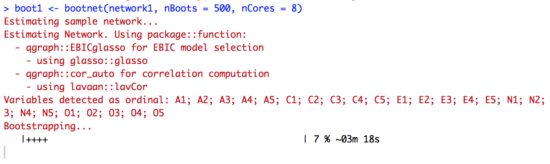
network1 <- estimateNetwork(bfi[,1:5],  default = "glasso")
boot1 <- bootnet(network1, nBoots = 500, nCores = 8)
plot(boot1, plot = "interval", split0 = TRUE, order="sample", labels=FALSE)

The above code will lead to a few warnings (ignore for the purpose of this tutorial³), and leads to the following figure:

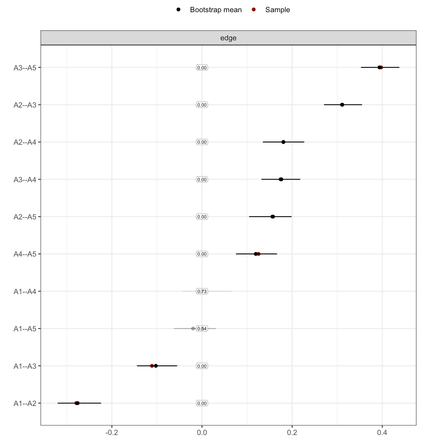
The saturation is proportional to how often an edge was included in the network. The figure doesn’t scale too well at present (i.e. to more than 5 or 10 nodes), but it’s something you’d likely report in the supplementary materials anyway, and not in the main part of your paper.

Thanks to Sacha and Jonas for the work they’ve put into this. Oh, and you know what’s also new? Bootnet estimates and tells you how long your coffee break should be 😉 …

1. For an explanation of regularization, see our tutorial paper
2. This is not the full plot, I omitted parts of it for the sake of legibility
3. See here for details