Tutorial: how to review psychopathology network papers

The network literature on psychopathology is exploding, which means there are many reviews to be performed. While each paper is different, some common themes have emerged, and because I have been asked on which aspects I focus my reviews and what my current main concerns are, here is a brief list of 10 topics and challenges papers should aim to navigate:

1. The nature of the investigated sample
2. Item variability
3. Selection effects and heterogeneity
4. Appropriate correlations among items
5. Publish your syntax and some important output
6. Item content
7. Stability
8. Properly interpreting centrality statistics
9. Considerations for time-series models
10. Further concerns and new developments

My main focus here is on network papers based on between-subjects cross-sectional data, although some of the points below also apply to within-subjects time-series network models. Note that these are all personal views, and I am sure other colleagues focus on other aspects when they review papers. Feedback or comments are very welcome.

1. The nature of the investigated sample

In the structural equation modeling (SEM) literature, researchers often investigate the factor structure of instruments that screen for psychiatric disorders. Frequently, data come from general population samples which predominantly consist of healthy individuals. This means that a conclusion such as “we identified 5 PTSD factors” seems difficult to draw, seeing that only few people in the sample actually met the criteria for a PTDS diagnosis.

The same holds for network models: I have reviewed many papers recently that draw inferences about the network structure of depression, or about comorbidity, but they investigate largely healthy samples. I don’t think that’s a good idea for somewhat obvious substantive reasons: don’t draw conclusions about a disorder if you don’t study patients with that disorder. But there are also two statistical reasons why the above may be a challenge, to which I will get below.

One argument against my position is that when we study intelligence or neuroticism in SEM, we investigate the factor structure of these constructs in broad samples, and don’t focus on populations of very intelligent or very neurotic people. That is true, and in that sense what you should do here depends a bit on how you understand a given mental disorder. If you think depression is a continuum between healthy and sick, with a somewhat arbitrary threshold, maybe you’re ok studying a general population samples to draw conclusions about depression. If you think depressed people are those with a DSM-5 diagnosis of depression, it may make less sense if you study depression when only 5% of your sample meet these criteria. My main point is that as a reviewer, I’d like to see that you think about this problem.

2. Item variability

Community samples may have very low levels of psychopathology, which can make the study of psychopathology in such samples difficult. If the item means are too low, the variability of the items becomes very small, and that can lead to estimation problems (an item without variability will not be connected in your estimated network because it cannot covary with other items). Note that technically this is not really an estimation problem – you can estimate your network just fine – but you may want to be aware of this when interpreting your network. I wrote a brief blogpost about this topic recently inspired by a paper from Terluin et al. where you can find more information.

The same problem can occur in samples with very severe levels of psychopathology or in case you have selection effects. For instance, we recently submitted a paper where the sample consisted of patients with very severe recurrent Major Depression. The mean of the “Sad Mood” item was 0.996 (item range 0-1), so we decided to drop it from the network analysis. Another example is the PTSD A criterion that states: “trauma survivors must have been exposed to actual or threatened death, serious injury, or sexual violence”. It makes little sense to include this item in a network analysis of PTSD patients because every person endorses this item, and it would show (partial) correlations of zero with other items.

Independent of what populations you study, differential item variability can pose a challenge to the interpretation of networks (items with low variability will unlikely end up being central items); that is, if an item in your network has a low variability and low centrality, it’s not clear if that item also would have a low centrality in a population in which it has a variability comparable to the other items. So I recommend you always check and report both means and variances of all your items. This can also be a problem when you, for instance, compare healthy and sick groups with each other. Multiple papers have now found that the connectivity or density of networks in depressed populations is higher than in healthy samples; connectivity is the sum of all absolute edge weights in a network. But this may be driven by differential variability: in healthy samples, the standard deviations of items will be smaller, which means items cannot be as connected as they are in the depressed sample.

3. Selection effects and heterogeneity

A second problem with studying mental disorders in healthy people is that there are good reasons to assume that the factor or network structure of psychopathology symptoms differs between healthy and sick people. We have found very convincing and consistent evidence for this phenomenon in Major Depression, across four different rating scales and two large datasets. And there are also good substantive reasons why this could be the case (e.g. 1, 2, 3).

In healthy samples, you may thus often end up drawing conclusions – for instance about the dimensionality or network structure of depression or PTSD symptoms – that would not replicate in a sample of depressed or traumatized patients.

Related to this is the problem of selection or conditioning on sum-scores. This is a tricky problem, and I’ve been trying to wrap my head around this for over a year now. Essentially, if you select a subpopulation (e.g. people with depression) on a sum-score of items that you then put into a network, you get a biased network and factor structure. This is shown analytically in a great paper by Bengt Muthén 1989 to which Dylan Molenaar pointed me a few months ago. This also holds for other psychological constructs of course, such as personality or intelligence. [Update 2019: our preprint on this issue is online!]

Because questions come up repeatedly about this, here an example. First, we flip two coins 100 times — the two results of the coin flips are uncorrelated, the coins are independent. These are our two symptoms, and the 100 rows are our people. Second, we now only select results into our data that have a certain sum-score, i.e. the sum of the two coin flips has to be at least 1. This is exactly the same as selecting depressed patients into a clinical datasets based on having 5 symptoms, for instance — we condition on a sum-score (or collider). If we look at the correlation again between the two coins, it is now about -0.5: we have induced negative correlations.

 
set.seed(1337)
x <- rbinom(n=100, size=1, prob=0.5)
y <- rbinom(n=100, size=1, prob=0.5)
 
cor(x,y) 
 
df1<-as.data.frame(cbind(x,y))
df1$z <- df1$x+df1$y
df2 <- subset(df1, df1$z>0)
 
cor(df2$x,df2$y)

4. Appropriate correlations among items

It’s not always easy to decide what type of correlation coefficient is appropriate for what type of data. In psychopathology research, data are often ordered-categorical and skewed. There are different ways to deal with this type of data, and Sacha Epskamp recently asked the following tricky question to students in the Network analysis course at University of Amsterdam:

“Often, when networks are formed on symptom data, the data is ordinal and highly skewed. For example, an item ‘do you frequently have suicidal thoughts’ might be rated on a three point scale: 0 (not at all), 1 (sometimes) and 2 (often). Especially in general population samples, we often see that the majority of people respond with 0 and only few people respond with a 2. This presents a problem for network estimation, as such data is obviously not normally distributed. Which of the following methods would you prefer to analyze such highly skewed ordinal data?”

We see the following 3 possibilities:

1. You can dichotomize your data, but you will lose information.
2. You can use polychoric or Spearman correlations that usually deal well with skewed ordinal variables.
3. You can transform your data, for instance using the nonparanormal transformation. But that only works in certain cases.

Personally, I tend to dichotomize in case I only have 3 categories and items are skewed (e.g. this paper). With 4 or more categories, the polychoric correlation seems to work best, and there is also some unpublished simulation work showing this. What I want to see when I review papers is that researchers are aware of this problem, thought about it and tried to find out whether what they are doing with their data is ok. For instance, I usually do both polychoric and Spearman, and if there are dramatic differences, I have a problem I need to solve. Note that polychoric correlations have problems if there are too few observations in cross-tables, which can sometimes lead to spurious negative edges; in these cases, Spearman does better. We discuss this here in more detail.

5. Publish your syntax and some important output

What you can always deposit online, or publish as supplementary materials, is your R code. This will make your results reproducible. What you also should publish are the means and standard deviations of your items. In the best case, you can simply publish your data, but that is often not possible. If you have ordinal or metric data, you can make your networks reproducible by publishing the covariance matrix of your items (because we use this matrix as input when we estimate the Gaussian Graphical Model). In case of the Ising Model, we need the raw data to estimate the network model, so without data your network will not be reproducible. However, you can still publish your model output (i.e. the edges and threshold parameters) so that your graph itself becomes reproducible, and you can also publish the tetrachoric correlations among items for some more insights.

6. Item content

I have only recently come to pay attention to this more, but it seems important to consider the content of the instrument you want to investigate as a network of items. That sounds both obvious and vague, but in some of my prior work, I simply threw all items of a rating scale into a network analysis. For instance, consider this network from a paper we published on bereavement:

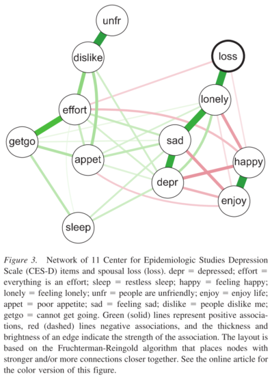
Thinking about this now, it seems that sad mood and feeling depressed are fairly similar to each other: do we really want to include both in one network? Or would it be better to represent these items as one node, each by averaging them, or estimating a latent variable? Angélique Cramer and me wrote about this in more detail in a paper entitled “Moving forward: challenges and directions for psychopathological network theory and methodology” that is currently under revision:

“We see two remaining challenges pertaining to the topic of constituent elements: 1) what if important variables are missing from a system, and 2) what to do with nodes that are highly correlated and may measure the same construct (such as ‘sad mood’ and ‘feeling blue’)?“

You can find the relevant section on pp. 17-19. I don’t have a solution, but it seems an important topic to pay attention to, especially since we work with partial correlation networks, and I wonder what remains of the association between sad mood and e.g. insomnia after we partial out depressed mood and feeling blue.

7. Stability

We have written about this a lot in the past, so I will only briefly reiterate: please check the stability, accuracy, and robustness of your network models (blog post; paper). It really helps the editor and reviewers of the paper to gauge its relevance and implications, but also helps readers to get a better grasp of the results. Conclusions should be proportional to evidence that is presented, and robust models certainly help with stronger evidence. I also gave a short presentation about robustness at APS 2016, and you can find a whole collection of updated slides on network robustness in the online materials of the network analysis workshop we have just 2 weeks ago. [Update 2019: a second part of the stability blog post series can be found here].

8. Properly interpreting centrality statistics

I wrote this topic up in a blog post in the future (and then time-travelled to put it here).

9. Considerations for time-series models

I have only reviewed a few time-series papers, and other people are much better suited go give feedback here. A good start for state-of-the-art models, model assumptions, and pitfalls are recent papers by Kirsten Bulteel, Jonas Haslbeck, Laura Bringmann, and Noémi Schuurman.

10. Further concerns and new developments

You can find a number of additional concerns and topics I wonder about in our draft on challenges to the network approach [update 2019: published here], but these currently play do not a major role when I review papers. And maybe you’d like to add important concerns to the comments below. In general, please be careful with drawing causal inference from cross-sectional data, and keep in mind that between-subjects and within-subjects effects may be different from each other.

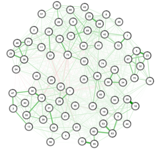
If you want to try out something novel that will hopefully become state-of-the-art in the next half year, check out the predictability metric that Jonas Haslbeck developed. This will result in something akin to R^2 of each node explain by all other nodes (indicated by the grey area around the nodes):

And it never hurts to have a research question of course: something you’re interested in, a hypothesis. I find network papers stronger and more interesting if it’s more than just applying

estimateNetwork(data, default="EBICglasso")

to a new dataset or disorder. The same applies to SEM papers as well of course.

Make sure to also check out the tutorials published here that list some further challenges I point out in reviews, such as problematic visualizations, centrality overinterpretation, issues with community detection, and others.

Some of these concerns come from discussions with colleagues such as Sacha Epskamp, Angélique Cramer, Denny Borsboom, Jonas Haslbeck, Claudia van Borkulo, Kamran Afzali, and Aidan Wright. So kudos to them and all other colleagues who commented on this blog post, and who have helped me grasp these issues in the last 2 years.